Understanding ML executions

As data scientists, the ability to comprehensively understand and monitor machine learning executions is paramount for delivering successful and impactful models.

This page is a resource that equips data scientists with the necessary knowledge and tools to track, monitor, and analyze the executions of their machine learning models on the Craft AI platform.

This page delves into essential topics, including obtaining execution details, tracking input and output, accessing metrics and logs, and comparing multiple executions. By mastering these techniques, data scientists can make informed decisions, optimize their models, and unlock the true potential of the MLOps platform.

Info

On this page, we will focus more on the pages available in the web interface. We'll mention the SDK functions available without going into detail about them.

Topics

• How to find an execution and obtain the details ?
• How to compare multiple execution ?
• How to follow a pipeline in production ?

Prerequisites

Before using the Craft AI platform, make sure you have completed the following prerequisites:

1. Get access to an environment
2. Connect the SDK
3. Create a step & pipeline
4. Execute this pipeline

On this page, we're going to focus on execution analysis using the platform's web interface. For the example, I'm going to use a basic deep learning use case to visualize the associated information. You can use your own use cases, of course.

Step code used in parts 1 and 2 (model training):

import tensorflow as tf
from tensorflow.keras import layers, models
from tensorflow.keras.datasets import fashion_mnist
from craft_ai_sdk import CraftAiSdk

def trainer(learning_rate=0.001, nb_epoch=5, batch_size=64) : 

    sdk = CraftAiSdk()

    # Load and preprocess the MNIST dataset
    (train_images, train_labels), (test_images, test_labels) = fashion_mnist.load_data()
    train_images = train_images.reshape((60000, 28, 28, 1)).astype('float32') / 255
    test_images = test_images.reshape((10000, 28, 28, 1)).astype('float32') / 255
    train_labels = tf.keras.utils.to_categorical(train_labels)
    test_labels = tf.keras.utils.to_categorical(test_labels)

    # Build the neural network model
    model = models.Sequential()
    model.add(layers.Conv2D(32, (3, 3), activation='relu', input_shape=(28, 28, 1)))
    model.add(layers.MaxPooling2D((2, 2)))
    model.add(layers.Conv2D(64, (3, 3), activation='relu'))
    model.add(layers.MaxPooling2D((2, 2)))
    model.add(layers.Conv2D(64, (3, 3), activation='relu'))
    model.add(layers.Flatten())
    model.add(layers.Dense(64, activation='relu'))
    model.add(layers.Dense(10, activation='softmax'))

    # Compile the model
    model.compile(optimizer=tf.keras.optimizers.Adam(learning_rate=learning_rate),
                loss='categorical_crossentropy',
                metrics=['accuracy'])

    # Train the model
    for epoch in range(nb_epoch):  # Set the number of epochs
        model.fit(train_images, train_labels, epochs=1, batch_size=batch_size, validation_split=0.2)

        # Evaluate the model on the test set and log test metrics
        test_loss, test_acc = model.evaluate(test_images, test_labels)
        print({'epoch': epoch + 1, 'test_loss': test_loss, 'test_accuracy': test_acc})
        sdk.record_list_metric_values("test-loss",  test_loss)
        sdk.record_list_metric_values("test-accuracy", test_acc)


    # Evaluate the model on the test set
    test_loss, test_acc = model.evaluate(test_images, test_labels)
    print(f'Test accuracy: {test_acc}')
    sdk.record_metric_value("accuracy", test_acc)
    sdk.record_metric_value("loss", test_loss)

    # Save the model
    model.save('mnist-model.keras')
    sdk.upload_data_store_object('mnist-model.keras', 'product-doc/mnist-model.keras')

Step code used in part 3 (inference with the model):

import tensorflow as tf
from tensorflow.keras.models import load_model
from PIL import Image
import numpy as np
from craft_ai_sdk import CraftAiSdk
import tensorflow as tf
from tensorflow.keras.datasets import fashion_mnist

def inference(image_num, model_path):

    sdk = CraftAiSdk()
    ima_path = './image_from_fashion_mnist.jpg'

    # Load the Fashion MNIST dataset
    (train_images, train_labels), (vali_images, vali_labels) = fashion_mnist.load_data()

    # save 1 image of validation dataset 
    image_to_save = Image.fromarray(vali_images[image_num]) 
    image_to_save.save(ima_path)    


    # Save model in local context and load it
    sdk.download_data_store_object(model_path, "model.keras")
    model = load_model("model.keras")


    # Preprocess the input image
    input_image = tf.keras.preprocessing.image.load_img(ima_path, target_size=(28, 28), color_mode='grayscale')
    input_image = tf.keras.preprocessing.image.img_to_array(input_image)
    input_image = np.expand_dims(input_image, axis=0)
    input_image = input_image.astype('float32') / 255.0

    # Make predictions
    predictions = model.predict(input_image)

    # The predictions are probabilities, convert them to class labels
    predicted_class = int(np.argmax(predictions[0]))

    if vali_labels[image_num] : 
        if vali_labels[image_num] == predicted_class:
            sdk.record_metric_value("score", 1)
        else :
            sdk.record_metric_value("score", 0)

    return {"predicted_class": str(predicted_class)}

How to find an execution and obtain the details ?

When using the platform for experimentation or production, you can find the list of all your executions on the Execution > Execution Tracking page (remember to select a project first).

On this page you will find the list of all executions in all environments of the selected project. All executions are listed, whether in progress, failed or finished, whether triggered by a run, endpoint or CRON.

Warning

Please note that deleting the pipeline or deployment will delete all attached executions.

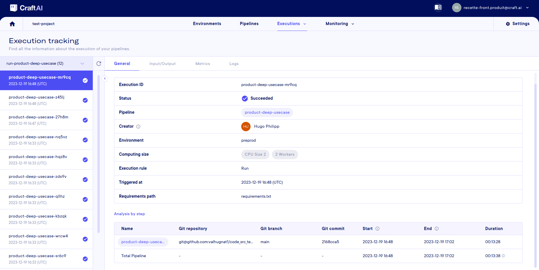
Get general information on an execution

Once you are in the execution tracking page, you need to select an environment using the selector at the top left. Once the mouse is over the environment, you will see another popup on the right with two lists in a row:

• The first contains the list of pipelines that have 'run' attached to them.
• The second contains the list of deployments that have executed attached to them.

Once a pipeline or deployment has been selected, the list of executions appears in the left-hand column, from the most recent to the oldest.

Tip

You can click on an environment directly to get all the associated executions.

Info

You can also retrieve all this information using the sdk.get_pipeline_execution(execution_id) function via the SDK.

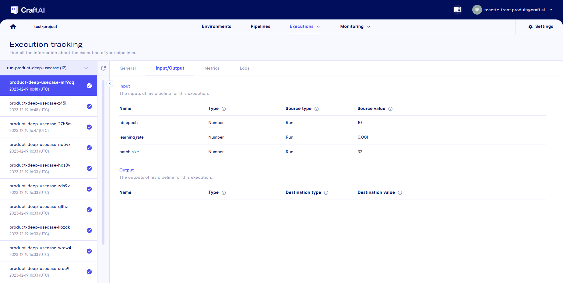
Track input and output of execution

If you want to see the inputs and outputs of a execution, you can view them in the tab of the same name. The inputs/outputs of the pipeline are displayed in a table with their:

• Name
• Type
• Source/destination type (where the value entered for this execution comes from)
• Source/destination value (what is the value entered for this execution)

Info

For the SDK, this information can be obtained using the function mentioned above sdk.get_pipeline_execution(execution_id).

More information can be obtained using the:

• sdk.get_pipeline_execution_input(execution_id, input_name)
• sdk.get_pipeline_execution_output(execution_id, output_name)

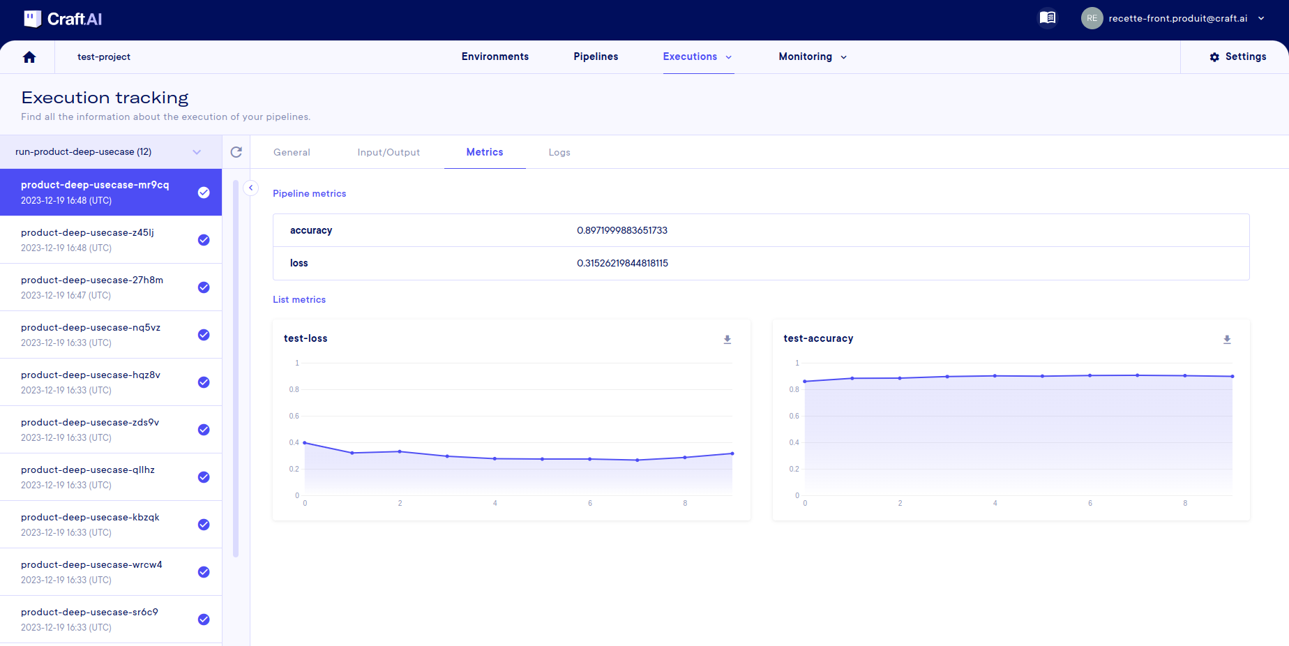
Get metrics and logs of execution

In the metrics tab, you can retrieve the pipeline metrics if you have defined them in your code.

Note that the 'simple metrics' are shown in a table, but the 'lists metrics' are shown with graphs so that you can see how they change during execution. For example, here we follow the evolution of loss and accuracy over the epochs of our model training.

Info

It is also possible to retrieve this information from the SDK using the functions sdk.get_metrics(name, pipeline_name, deployment_name, execution_id) and sdk.get_list_metrics(name, pipeline_name, deployment_name, execution_id), more information here.

Finally, the execution logs are also available in the associate tab. Note that the logs, like the other information, are not automatically reflected in the web interface, hence the buttons with arrows for refreshing the page.

Info

Here again, an SDK function is available with sdk.get_pipeline_execution_logs(pipeline_name, execution_id, from_datetime, to_datetime, limit).

How to compare multiple executions?

Compare execution with a table of comparison

Let's go back to the source code of the step from the beginning. This code is designed to train a deep learning model. This model has three hyper-parameters (the learning rate, the number of epochs, and the batch-size) which are associated with inputs to the step.

We can also see that in the step code, there are simple metrics and lists to track performance during and at the end of training.

Here, we'll vary the hyperparameters over several training sessions to find the best values. We'll vary the learning rate and batch size with these values:

Learning rate	Number of epochs	Batch size
0.01	10	32
0.01	10	64
0.01	10	128
0.001	10	32
0.001	10	64
0.001	10	128
0.0001	10	32
0.0001	10	64
0.0001	10	128

Each line in this table represents an execution with its hyper-parameters and therefore a training run of the model.

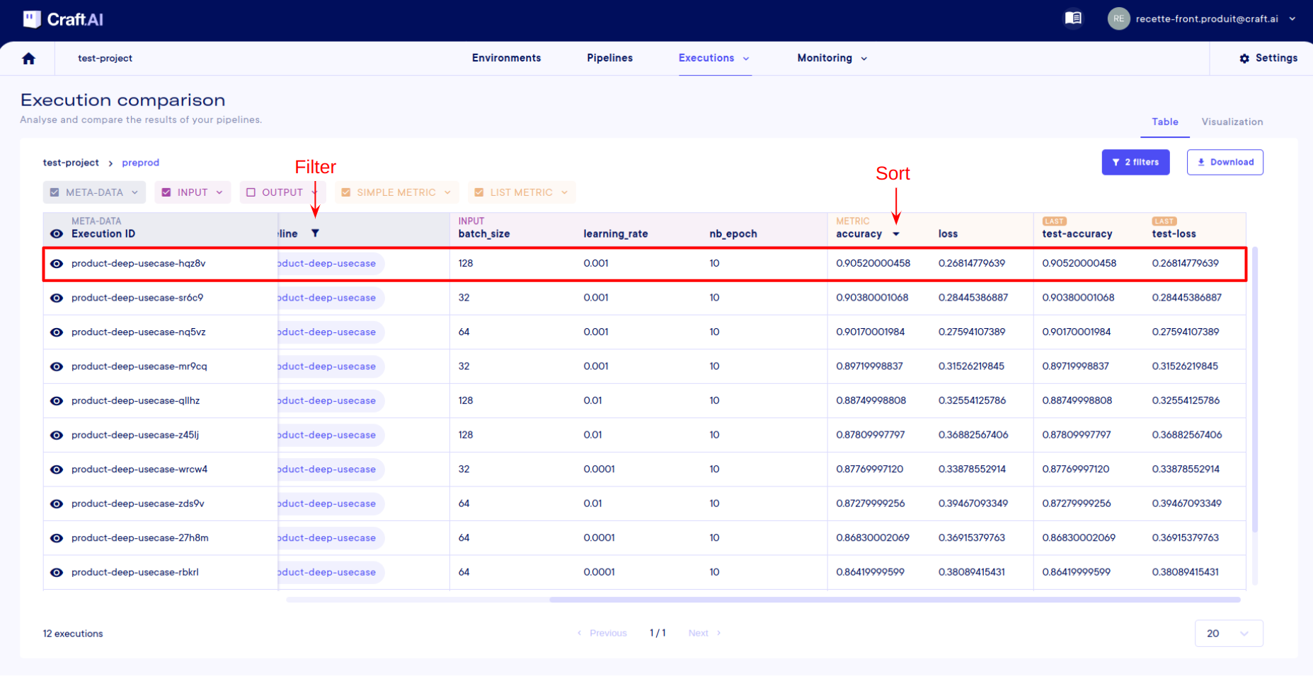
Instead of looking at the executions one by one in execution tracking, we go to Executions > Execution Comparison. Then select its environment, to finally see the table with all the executions.

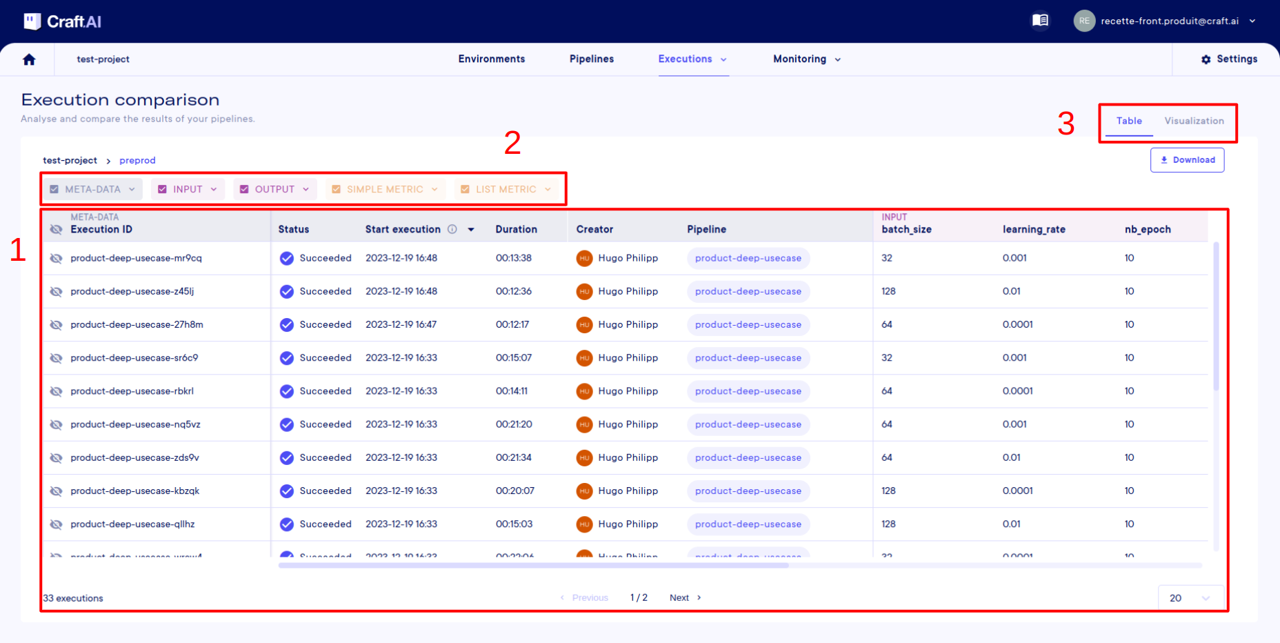
There are 3 important elements on this page:

1. The table, the central element of the page. In this table, each row represents an execution, except for the first row, which is the column header. Each column represents information about the executions.
2. These selectors can be used to add more or less information to the table, allowing inputs, metrics, etc. to be displayed or not. The more information you select, the more columns the table will have.
3. Another tab is available on this page for viewing the metrics lists, but we'll come back to this later.

To start with, I'm going to select the meta-data, inputs, simple metrics, and list metrics. We don't need the outputs in this case. If I want, I can even select precisely the inputs and metrics I've used in my executions.

Then, in the header of the table, I'll filter the pipeline names so that I only have the executions from the pipeline I've used.

Note

All filter settings are available from the Filters button at the top right of the screen.

Finally, I'll sort according to precision by clicking on the little arrow in the column header.

That's it, I've sorted my executions to find the parameters that give me the best accuracy for my model. In my case, the best result is obtained with a learning rate of 0.001 and a batch size of 128.

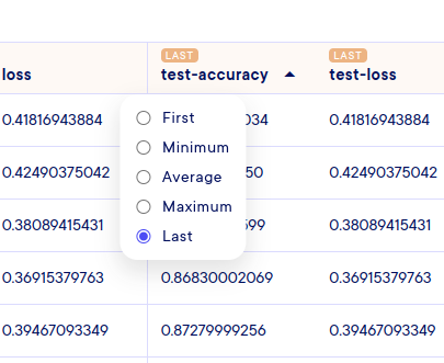
We could also have sorted according to metric lists, with the difference that you have to select your calculation mode before sorting. In fact, since we're just displaying a number representing the list (with the average, the last number, the minimum, etc.), you do this by clicking on the tag at the top of the column (here with last in the screenshot below):

CCompare the list metrics of several executions

If you want to see all the values in the execution lists, you can also display the list metrics in their entirety to compare them between executions. To do this, select the executions you want to view using the eye on the left of the table, then go to the visualize tab (top right).

Note

Only list metrics executions have a selectable eye.

On this screen, there is a graph for each available metrics list, and each execution is represented by a color. So you can compare the evolution of your metrics between each training session.

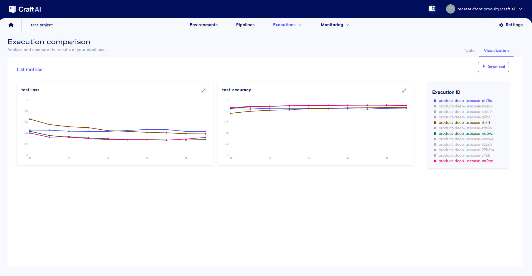
Info

You can hide executions by clicking on their names in the legend.

How to follow a pipeline in production?

Pipeline monitoring

Once our model has been trained and selected, we're going to expose it in an endpoint so that it can be used from any application. To do this, we're already going to need source code for an inference pipeline, this is the 2ᵉ Python code given at the beginning. Note that this code reuses the validation dataset, to do the inference, for simplicity. We can, therefore, score each prediction and put the result in a score metric:

• 1: The prediction is accurate
• 0: The prediction is false

We create the step, the pipeline, and the endpoint deployment with the associated input/output. Our model is now ready to make predictions. For each prediction, we can track executions using the tools we've already seen.

In addition, you can also monitor our executions more globally over time by going to Monitoring > Pipeline metrics. On this page, you can see the evolution of the single metrics over time for any selected deployment.

In our case, we can track, execution after execution, the prediction score (true or false) of the model:

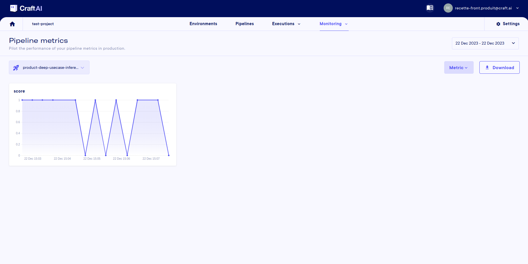
Info

You can select a date range in the top right-hand corner. You can also zoom in on a selected range in the graph.

Resource monitoring

When you have several models in production (or even in training), you may want to have information about the health of your environment's infrastructure. This helps to ensure that the size of the environment corresponds to the computation/storage requirements and also to identify any problems.

The Monitoring > Resource metrics page allows you to see any over-use of resources (with the cards at the top), as well as their evolution over time (with the graphs), once an environment has been selected.

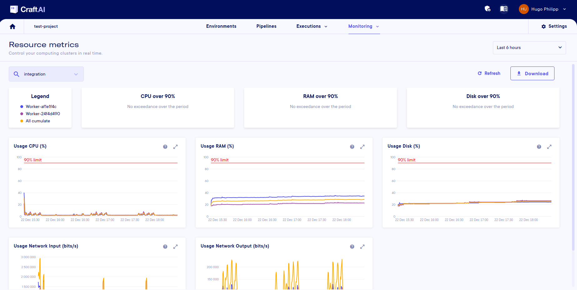
As a reminder, an environment is made up of workers, which are the calculation units within the environment. Each worker, therefore, has a dedicated curve (selectable from the legend) plus a curve for all the cumulative workers.

You can download this data in .csv format using the download button. The data downloaded will be that selected by date and worker (as for the graphs).

Info

It is also possible to retrieve data with the SDK using the sdk.get_resource_metrics(start_date, end_date, csv) function.

The csv (binary) parameter can be used to retrieve data in .csv format, like the button, or in a Python dictionary.

Conclusion

In this page, we have covered essential aspects of tracking, monitoring, and analyzing machine learning executions on the Craft AI platform. By understanding how to find and obtain details about executions, track input and output, retrieve metrics and logs, and compare multiple executions, data scientists can effectively leverage the platform's capabilities.

Additionally, we explored the process of following a pipeline in production, including pipeline monitoring and resource monitoring. These practices ensure that models are deployed and running smoothly, with the ability to assess performance and resource utilization over time.

By mastering these tools and techniques, data scientists can make informed decisions, optimize models, and achieve the full potential of the MLOps platform provided by Craft AI.